E.T.C.
On this page I introduce the simulation tools I have built so far. Since there is no uniformity in the genres, I have grouped them all together under "etc." :-). I've been updating quite frequently recently. I'm not sure how long I can keep up these updates, but I'd like to keep trying as long as I'm still interested. The tools I've introduced are as follows:
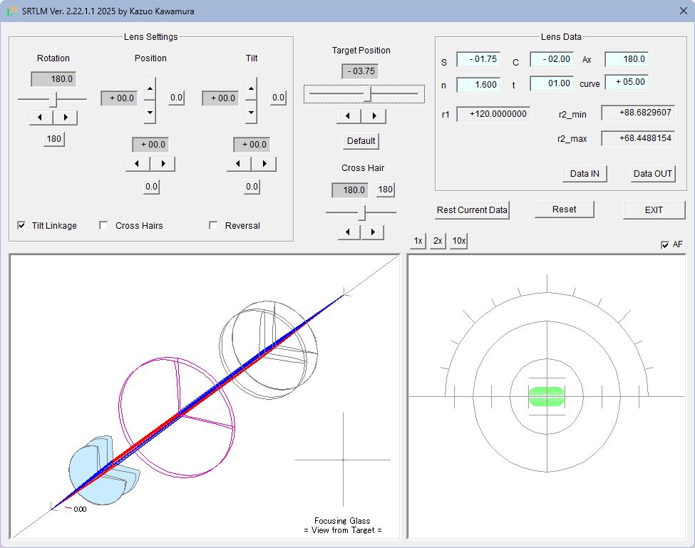
Lens Meter Simulation tool =SRTLM=
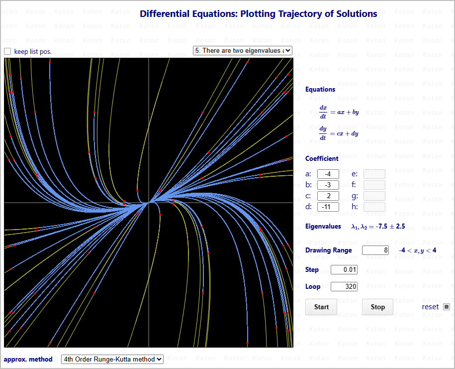
Differential Equations drawing tools
Rendering Surfaces with Hidden Line Meshes
Voyagers of 38,000 years ago
Here is a list of the tools I have introduced, presented in the order they were released or updated:
List view of update history
▽
- 26/04/12 Differential Equation Visualization Tool (3D): Added new equations
- 26/03/19 Differential Equation Visualization Tool (2D): Added vector field display function
- 26/02/15 Differential Equation Visualization Tool (2D): Improved calculation logic for initial points
- 25/11/23 Lensmeter Simulation Tool "SRTLM": Updated
- 25/10/13 Lensmeter Simulation Tool "SRTLM": Source code released
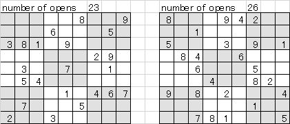
- 25/09/24 Sudoku Puzzle Generator Tool: Released alternative solving method”
- 25/09/24 Sudoku Puzzle Generator Tool: Updated
- 25/09/24 Sudoku Puzzle Generator Tool: Released
- 25/03/26 Voyagers of 38,000 years ago: Released
- 24/09/08 Surface Rendering Tool: Released
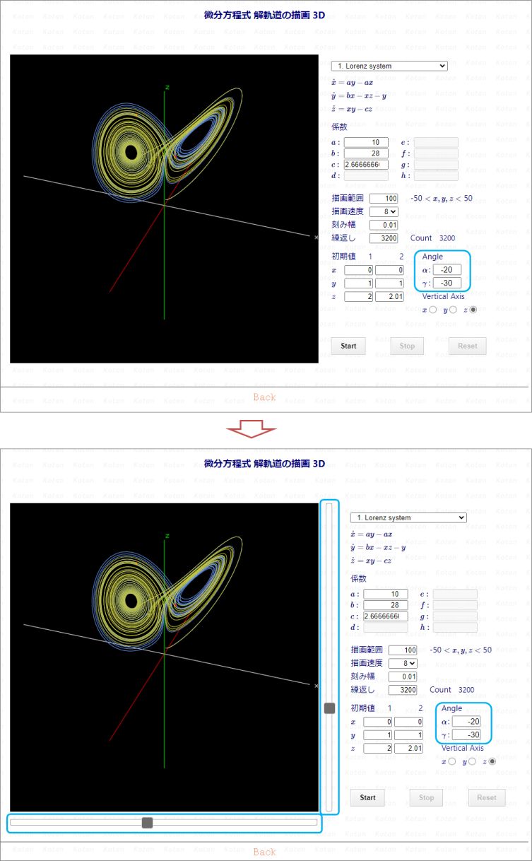
- 24/07/06 Differential Equation Visualization Tool (3D): Added slider bar to improve usability
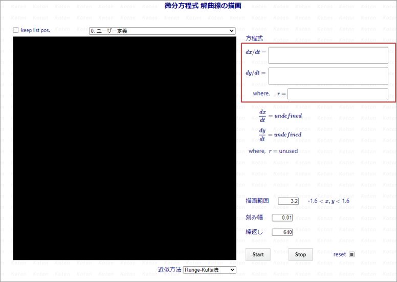
- 24/06/24 Differential Equation Visualization Tool (2D): Added user input function for equations
- 24/05/11 Differential Equation Visualization Tool (2D): Added equations (Part 4)
- 24/04/28 Differential Equation Visualization Tool (2D): Added equations (Part 3)
- 24/04/15 Differential Equation Visualization Tool (2D): Added equations (Part 2)
- 24/03/23 Differential Equation Visualization Tool (2D): Added equations (Part 1)
- 24/03/03 Differential Equation Visualization Tool (2D): Released
- 24/03/03 Differential Equation Visualization Tool (3D): Released
- 23/08/01 Lensmeter Simulation Tool "SRTLM": Released
04/15/26

I have added the following equations to the page
that plots solution trajectories for differential equations (3D).
- [08] Chen-Lee system
- [09] Chen system
- [10] Chua system
- [11] Langford system
- [12] Dadras system
03/19/26

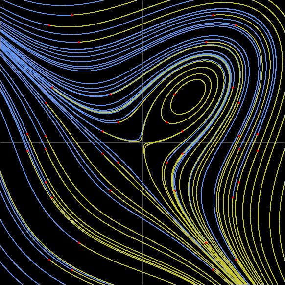
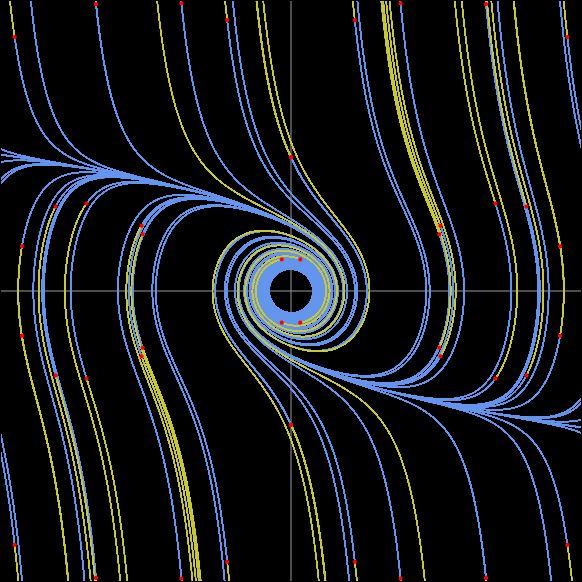
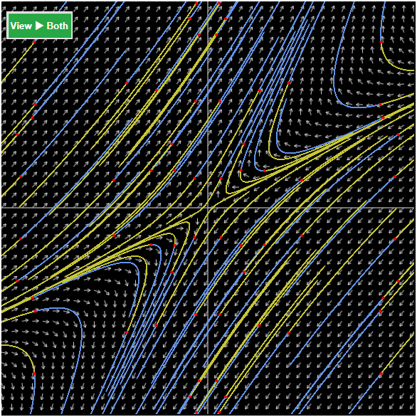
I have added a vector field display to the page
that plots solution trajectories of a two-dimensional differential equation.
A [View ▶ Traj] button has been added to the right of the [start], [stop], and reset[ ] buttons
in the upper right corner of the screen.
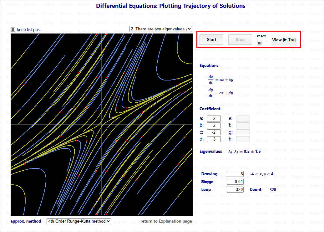
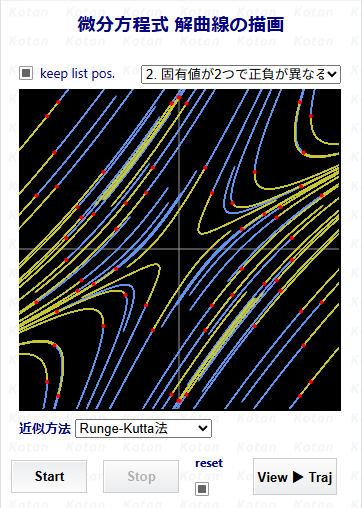
A [View ▶ Traj] button has been added to the right of [start], [stop], and reset[ ]
below the drawing window.
This button is a toggle; pressing it changes the display as shown below.


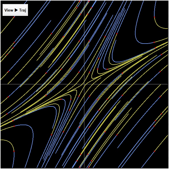
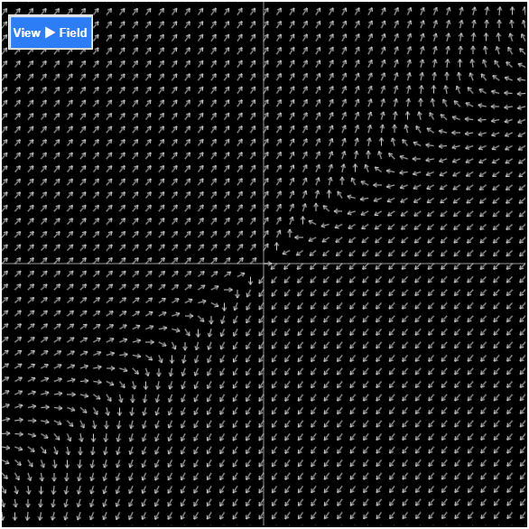
Below is link to explanatory page:
Clicking "To Plot" in the explanation section of each equation will transition you to the drawing page with the necessary data set for plotting. Clicking the [START] button begins plotting the solution curves.
Clicking "To Plot" in the explanation section of each equation will transition you to the drawing page with the necessary data set for plotting. Clicking the [START] button begins plotting the solution curves.
The following link directly jumps to the drawing page:
Select an equation from the dropdown box and click [Start] to begin plottinf the solution trajectory.
Select an equation from the dropdown box and click [Start] to begin plottinf the solution trajectory.
Refer to User defined Equations for details of the drawing page.
02/15/26

In the page for drawing the solution trajectory of a differential equation (2D),
there was an issue with the logic for drawing the initial value of the solution trajectory,
which resulted in the initial value sometimes exceeding the drawing range. This has been fixed.
Originally, it was programmed to give 16 initial values for each quadrant,
but I noticed that for some reason only 8 or 9 points were being given. After checking,
I found that the initial values sometimes were being given outside the drawing range,
so I corrected it.
Below is link to explanatory page:
Clicking "To Plot" in the explanation section of each equation will transition you to the drawing page with the necessary data set for plotting. Clicking the [START] button begins plotting the solution curves.
Clicking "To Plot" in the explanation section of each equation will transition you to the drawing page with the necessary data set for plotting. Clicking the [START] button begins plotting the solution curves.
The following link directly jumps to the drawing page:
Select an equation from the dropdown box and click [Start] to begin plottinf the solution trajectory.
Select an equation from the dropdown box and click [Start] to begin plottinf the solution trajectory.
Refer to User defined Equations for details of the drawing page.
11/23/25

Lens Meter Simulation Tool “SRTLM” has been updated.
Upon releasing the source code (10/23/25),
I checked the usability and made corrections to several points that concerned me.
For details, click the Lensmeter-Simulation-Tool below
and refer to "SRTLM_Correction_Update_History.txt."
The only visual change in the SRTML execution screen
is the addition of the “1.523” checkbox in the [Lens Data] section.

The front surface radius of the lens is calculated based on the “Curve” setting.
This checkbox provides the following options:
This checkbox provides the following options:
Check OFF: Use the refractive index of the tested lens for “curve” calculations (previous SRTLM specification).
Check ON: Use the traditional crown glass refractive index of 1.523 for “curve” calculations.
Check ON: Use the traditional crown glass refractive index of 1.523 for “curve” calculations.
Originally, “curve” refers to the front surface refractive power of a lens.
Therefore, if the lens's refractive power changes,
the same curve will have a different refractive power.
For example, taking a “5” curve as an example, it would be as follows.
| index | curve | radius |
|---|---|---|
| 1.500 | 5.0 | 100.0mm |
| 1.600 | 5.0 | 120.0mm |
| 1.700 | 5.0 | 140.0mm |
On the other hand, if the curve is represented with a refractive index of 1.523
regardless of the test lens's refractive index,
the front radius of the lens becomes constant regardless of the test lens's refractive index.
For example, for a "5" curve, it becomes "104.6mm".
If the "curve" uniquely represents the radius of the front surface of the lens,
it becomes much easier to match lenses with frames.
I added this feature because I believe it is necessary for handling the tool.
[E.T.C.] - etc_SRTLM_document_add_en
10/13/25

The source code for the lens meter simulation tool "SRTLM" has been released.
You can get it from GitHub by clicking "Lensmeter-Simulation-Tool" below.
For executable files and documentation, please refer to SRTLM_En as before.
[E.T.C.] - SRTLM_En
09/10/25

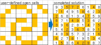
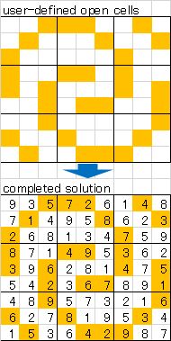
I have created an another version of the Sudoku puzzle generator tool using an Excel macro.
This another method allows you to create puzzles with freely defined patterns. And generate the completed form.
This another method allows you to create puzzles with freely defined patterns. And generate the completed form.
This tool can be downloaded as freeware.
[E.T.C.] - SudokuAnother Method
09/10/25

Updated the Sudoku puzzle generation tool: Added the ability to save generated puzzles.
This tool can be downloaded as freeware.
[E.T.C.] - Sudoku Update01
09/10/25

I have created a tool for generating Sudoku puzzles using an Excel macro.
This tool can be downloaded as freeware.
[E.T.C.] - Sudoku
03/26/25

For this site, this is a rather unique topic.
I seriously considered
"the mystery of the seafarers who transported obsidian by boat
from Kozushima Island in the Izu Islands to the mainland 38,000 years ago. "
[E.T.C.] - Voyagers of 38,000 years ago
09/08/24

I have released a page that plots graphs (surfaces) of functions of two variables
using a mesh with hidden line.
Select a function on the select box to plot the surface.
Below is link to explanatory page:
The following link directly jumps to the drawing page:
Select an function from the dropdown box and click [Start] to begin plot the surface.
[E.T.C.] - Plotting Surfaces Using Hidden Line Meshes
Select an function from the dropdown box and click [Start] to begin plot the surface.
[E.T.C.] - Plotting Surfaces Using Hidden Line Meshes
In addition to the pre-prepared functions,
the plotting page also has a feature that allows users to enter function directly and render graphs.
By entering the function you want to check, you can quickly check the shape of the surface.
07/06/24

On the page for drawing the solution trajectory of a differential equation (3D),
I have changed the operation using the spin button to a slider bar.
Previously, the coordinate system could be rotated after drawing using the spin button.
However, this was difficult to use, so we have modified it
so that it can be rotated smoothly using the slider.
06/24/24

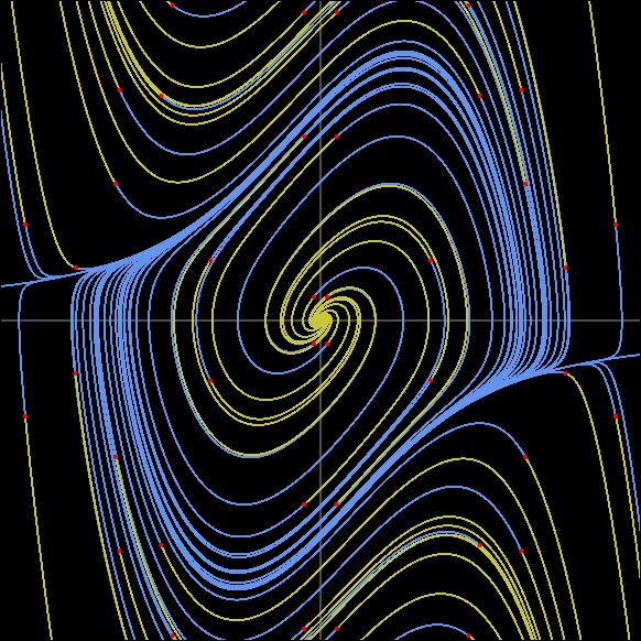
The following features have been added to the page for drawing solution trajectories of differential equations (2-dimensional).
Previously, the drawing page only allowed you to draw solution orbits for pre-set equations,
but by selecting "User Input", you can freely set equations.
You can quickly investigate the solution orbits, equilibrium points, etc.
of the equations you want to check.
This is a feature I personally wanted on the drawing page, so I hope you will find it useful.
Refer to User defined Equations for details.
05/11/24

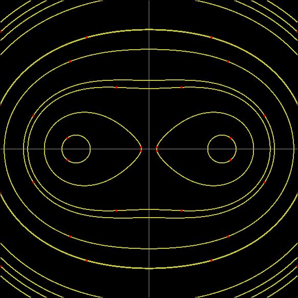
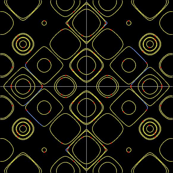
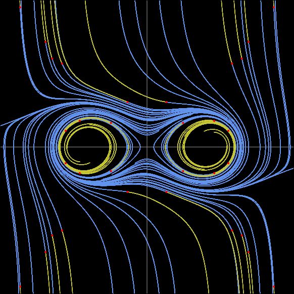
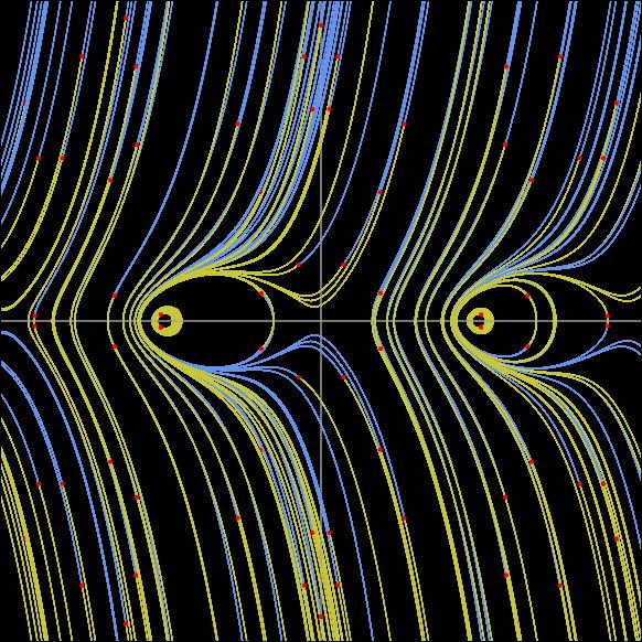
The following equation has been added to the page for drawing solution trajectories of differential equations (2-dimensional).
[04] 2-Dimensional Autonomous System Examples
- Hamilton system 1 : Cassini oval
- Hamilton system 2 : folium of Descartes
- Hamilton system 3 : derivatives of "folium of Descartes"
- Hamilton system 4 : Case of the periodicity of trigonometric functions is reflected
04/28/24

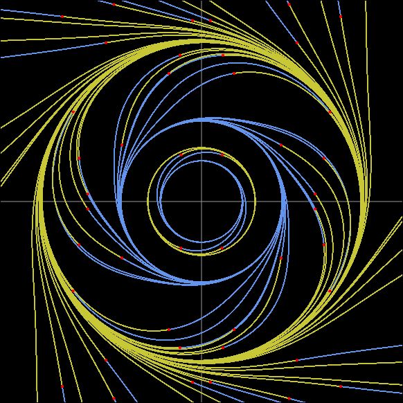
The following equation has been added to the page for drawing solution trajectories of differential equations (2-dimensional).
[04] 2-Dimensional Autonomous System Examples
-
Limit Cycle: example 4 Linear approximation with purely imaginary numbers - 1
Case of no limit circle exists -
Limit Cycle: example 5 Linear approximation with purely imaginary numbers - 2
case : an infinite number of limit circles appear
04/15/24

The following equation has been added to the page for drawing solution trajectories of differential equations (2-dimensional).
[04] 2-Dimensional Autonomous System Examples
- Limit Cycle Example 1
- Limit Cycle Example 2: von del Pol
- Limit Cycle Example 3: Lemniscate
03/23/24

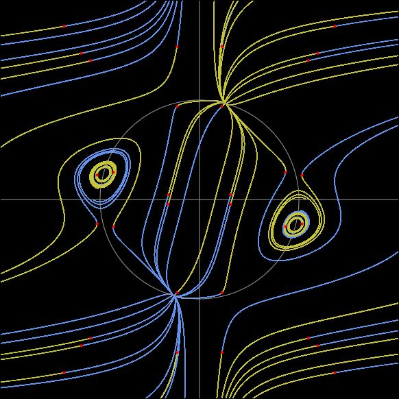
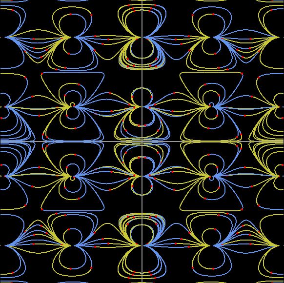
The following equation has been added to the page for drawing solution trajectories of differential equations (2-dimensional).
[04] 2-Dimensional Autonomous System Examples
- Autonomous system with periodic equilibrium points on x-axis
- Autonomous system with 8 equilibrium points on the circumference
- Autonomous system with 8 equilibrium points on a plane
03/10/24

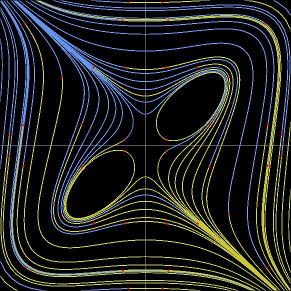
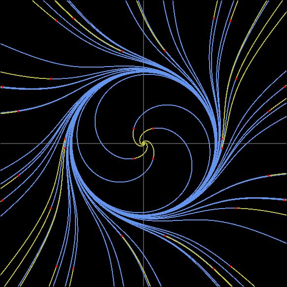
I have published a page for drawing solution trajectories of (2-dimensional) differential equations.
When you select an equation on the page, it dynamically plots the solution trajectory.
Originally, I had built a drawing tool in C#, but I wanted to directly draw on the web, so I rewrote it in JavaScript. However, I only had minimal experience with JavaScript about 10 years ago, and I encountered several "Hmm, how do I do this again?" moments.
So, I utilized ChatGPT. I want to explicitly mention here that using ChatGPT significantly saved me time in looking up things while coding.
The equations featured on this page are based on excerpts from
"Differential Equations on Personal Computers" by Mitsuo Morimoto.
Although Morimoto has introduced many equations, I haven't completed confirmation on my end yet.
Once confirmed, I intend to gradually add them.
Below is link to explanatory page:
Clicking "To Plot" in the explanation section of each equation will transition you to the drawing page with the necessary data set for plotting. Clicking the [START] button begins plotting the solution curves.
Clicking "To Plot" in the explanation section of each equation will transition you to the drawing page with the necessary data set for plotting. Clicking the [START] button begins plotting the solution curves.
The following link directly jumps to the drawing page:
Select an equation from the dropdown box and click [Start] to begin plottinf the solution trajectory.
Select an equation from the dropdown box and click [Start] to begin plottinf the solution trajectory.
On the drawing page, you can configure the following settings:
- Coefficients (modifiable parameters vary for each equation)
- Plotting range
- Increment width (width of elapsed time)
- Iteration count (number of executions of the increment width)
- Approximation method (Euler's method, Modified Euler's method, 4th Order Runge-Kutta method)
03/10/24

I have also published a page for plotting solution trajectories of differential equations with 3D.
It operates similarly to the 2D version of the differential equation page,
and I would like to note that I utilized ChatGPT in the same manner.
The equations showcased on this page primarily focus on chaotic trajectories.
If I find interesting equations, I plan to increase the samples.
Below are links to explanatory pages:
Clicking "To Plot" in the explanation section of each equation
will transition you to the drawing page with the necessary data set for plotting.
Clicking the [START] button begins plotting the solution curves.
After drawing, you can observe the solution trajectories from various angles by changing the Angle and Vertical Axis.
The following link directly jumps to the drawing page:
Select an equation from the dropdown box and click [Start] to begin drawing the solution trajectory. After drawing, you can observe the solution trajectories from various angles by changing the "Angle" and "Vertical Axis".
Select an equation from the dropdown box and click [Start] to begin drawing the solution trajectory. After drawing, you can observe the solution trajectories from various angles by changing the "Angle" and "Vertical Axis".
On the plotting page, you can configure the following parameters:
- Coefficients (a–h; note that these vary depending on the equation)
- Plotting range
- Increment width (width of elapsed time)
- Iteration count (number of executions of the increment width)
- Initial values (can specify 2 points)
- Angle (left-right, up-down)
- Vertical Axis (default is z-axis, but you can also choose x-axis and y-axis)
08/01/23

Lens meter simulation tool "SRTLM" has been released.
This tool can be downloaded as freeware.
[E.T.C.] - SRTLM_En


